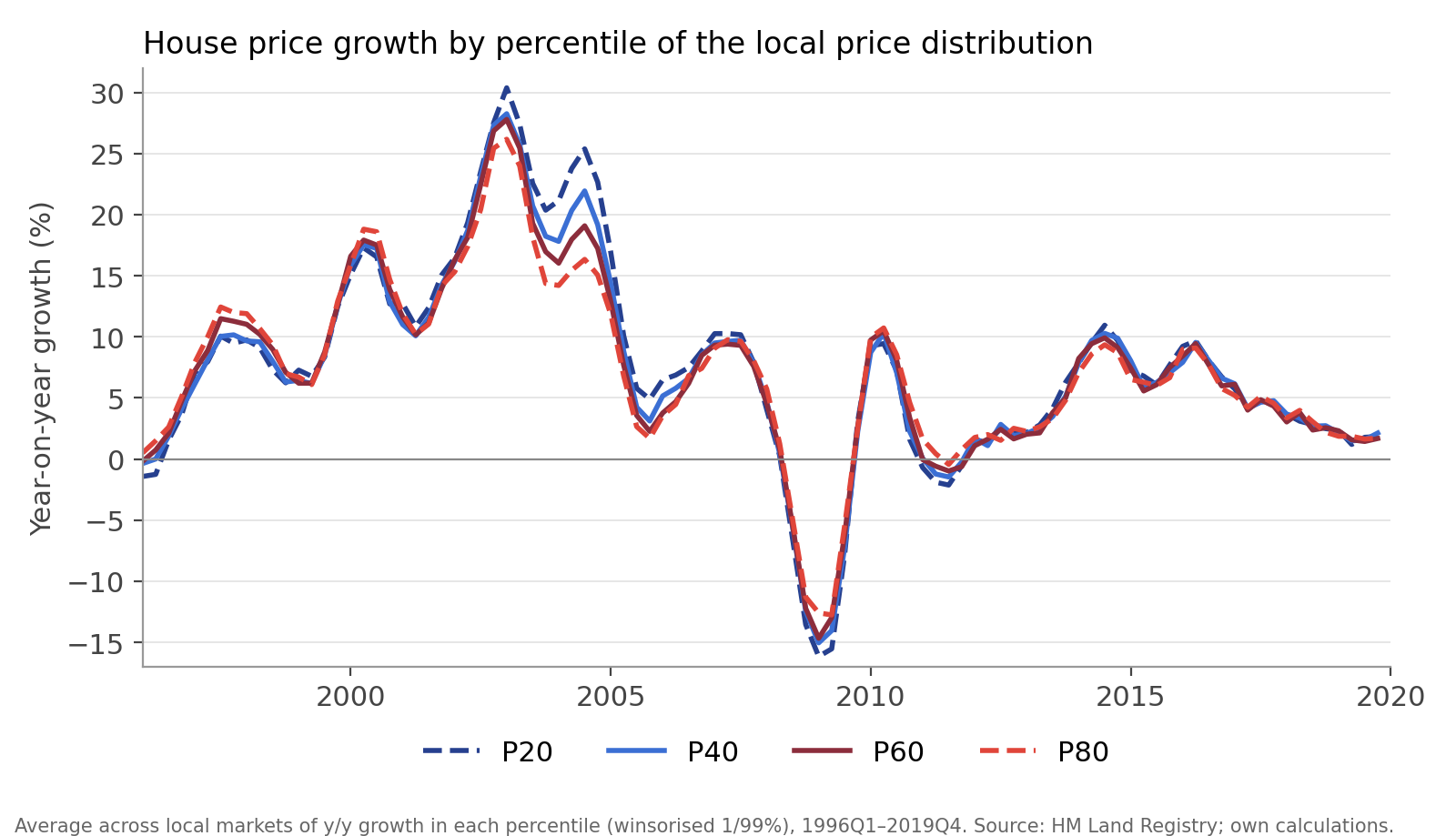
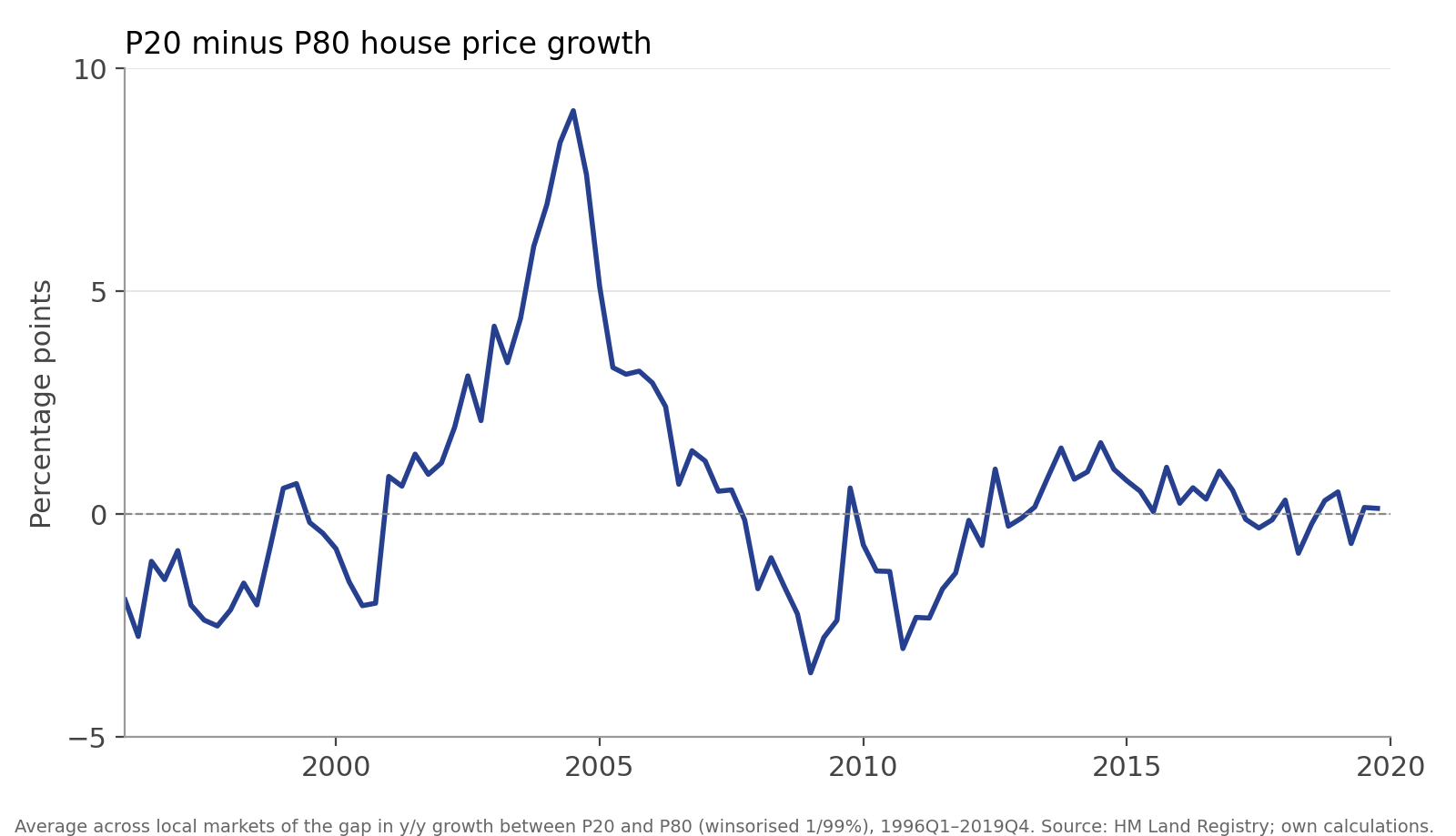
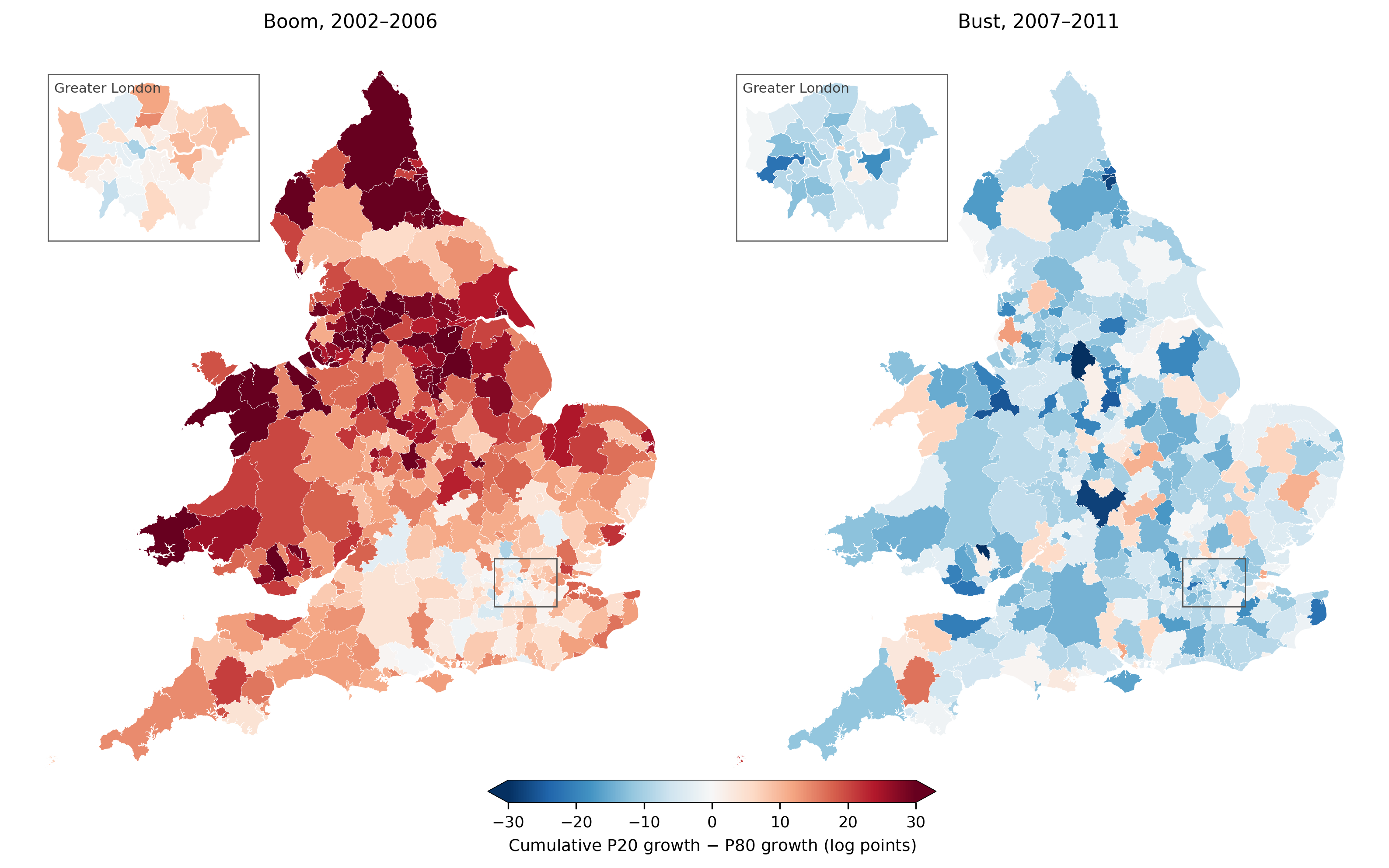
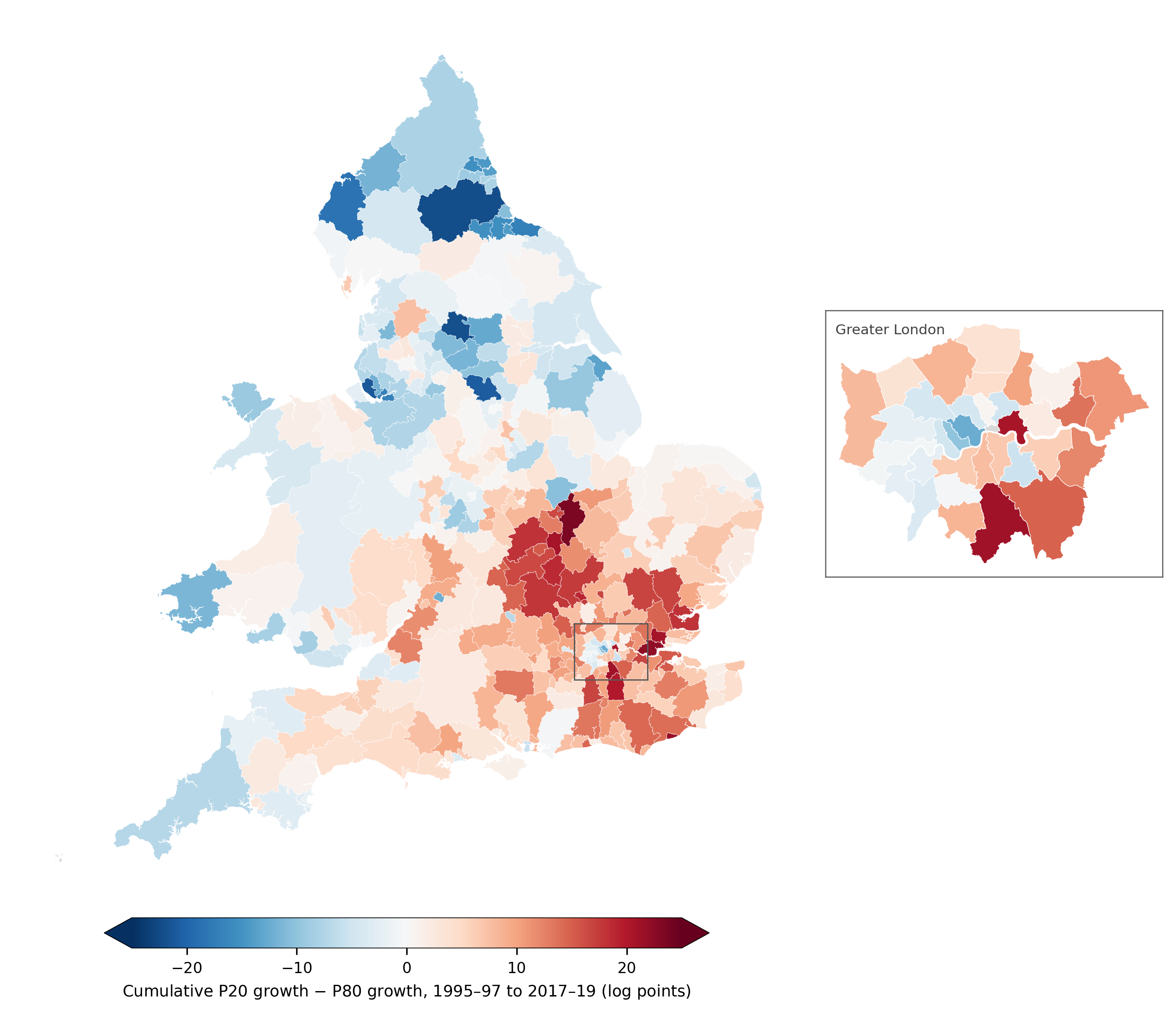
In the previous post, I discussed the building of the distributional house price indices (DHPIs) for the U.K., noting that they allow us to study something that is typically not possible with other house price indices: the within-local market heterogeneity in house price growth. In this second (and last) post, I will go through the main findings of the paper: the heterogeneity, in particular the differences between low- and high-priced houses, is systematic.
Before going there, however, let me mention something that is crucial for the analysis: all the results are within-market statements. In econometric terms, I use local area-by-quarter fixed effects. That means that shocks affecting areas are captured by these fixed effects. One question that comes from this approach is whether there is meaningful variation within markets. The answer is yes. A simple regression of house prices with local area-by-quarter fixed effects shows that most of the variation in house prices remain unexplained. So my approach controls for local-area trends while focusing on substantial variability.
The first question that I had from plotting the DHPIs was whether different parts of the house price distribution move differently depending on the position of the economic cycle. Using (lagged) real GDP growth, it turns out that they do: when GDP growth is high, lower-priced houses increase by more than higher-priced ones. The magnitude is important: a one standard deviation increase in GDP growth is associated with 0.46 percentage points higher price growth for cheaper houses compared to more expensive ones. What is also important is the monotonicity of this relation: as we move closer to the right of the price distribution, this heterogeneity dies down.
GDP growth is a measure of the economic cycle, but another one that might be more relevant is credit. Indeed, macroprudential regulators tend to look at measures of credit to understand whether they need to use macroprudential tools. So I repeat the same exercise using net secured lending flows, that is, how much new secured lending (basically mortgages) banks and other financial institutions provide minus the repayments during that quarter. The same relation appears, but with a twist: cheaper houses increase in prices by more when credit is high, but the magnitude is almost three times stronger than for GDP growth (1.24 vs. 0.46). Indeed, when we put both measures of the cycle together, the coefficient for GDP growth drops substantially and is no longer significant, while the coefficient for credit barely changes. In other words, the cycle that matters for the heterogeneity is the credit cycle.
That is all great (well, at least that’s what I think) but it is about correlations. Is the cycle causing the heterogeneity? You could construct an alternative story. For instance, when households in the lower-priced housing segment expect this segment to appreciate substantially, they borrow more, which pushes credit up, and subsequently are more likely to buy houses, pushing demand and prices up. It would be great to use exogeneous shocks instead. This is where monetary policy surprises come in.
Monetary policy decisions are extremely endogenous to the conditions of the economy. But these decisions are also incredibly consequential for businesses, financial institutions, households, and macroeconomic performance. So the literature has for many years now spent a lot of time trying to obtain monetary policy shocks. One of the most used approaches is using monetary policy surprises, that is, changes in yields around monetary policy announcements. This is what I use here, partly due to the availability of these shocks for the U.K. from Braun et al. (2023).
What should we expect if the channel is that higher credit availability leads to higher housing demand particularly for constrained borrowers, who are more likely to be in the cheaper segments? We should expect that higher interest rates are associated with lower price growth for cheaper houses. This is indeed what I find. Positive monetary policy surprises (that is, monetary policy announcements that revise yields up) reduce the price growth of cheaper houses compared to more expensive ones. The effect comes from changes in the short-end of the yield curve, rather than changes in longer-term yields, consistent with the channel coming through mortgage lending. I also show that the effect does not revert: the drop in price growth continues to accumulate for at least four years after the monetary policy shock.
There are other results and details that I cannot include in the blog, so I encourage anyone interested in the topic to look at the paper. Also, for the first time in my academic career, I have included a replication package on GitHub; perks of not using confidential data. This is just version 1; I am extending the analysis in two directions now: studying quantities and bringing local market heterogeneity. But so far, I think the results bring something that may not be well-known: within-market heterogeneity is substantial, and different price segments move systematically with the credit cycle. Importantly, monetary policy has distributional consequences within local markets through house prices, hitting lower-priced houses the hardest.