In the first post, I made the case for borrower-based tools: individually rational borrowing can be collectively excessive, and it can be optimal for the regulator to cap how much households can borrow against their homes. But I ended on a corollary: these tools affect some segments of the population disproportionally. This post explores some of the evidence of this unequal impact.

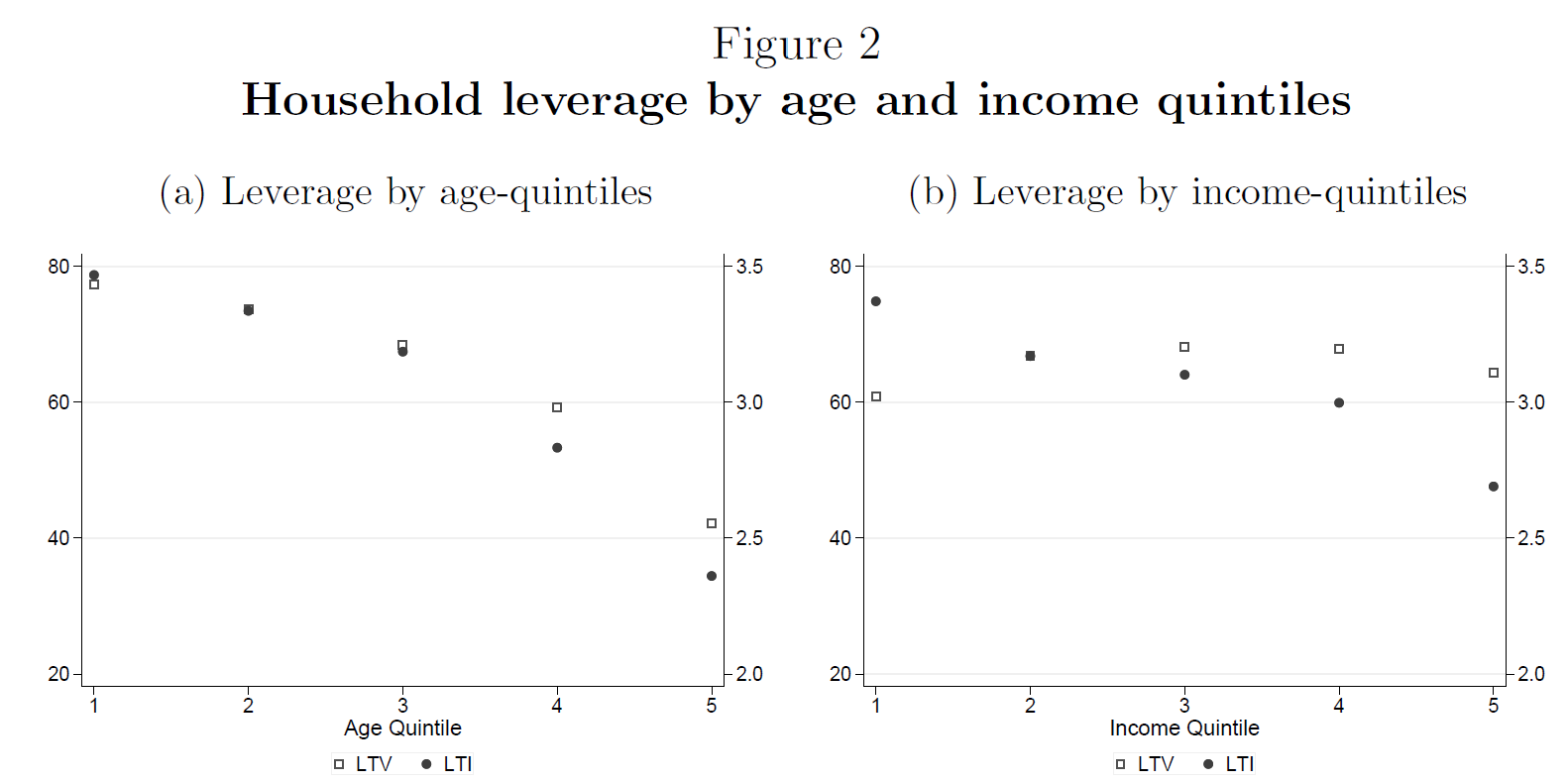
Leverage is not spread evenly across borrowers. If one looks at Figure 2 in our paper, reproduced below, we can see that both loan-to-value and loan-to-income ratios falling steadily with age and with income (particularly LTI). The people borrowing at the highest multiples are the young, the lower-income, the first-time buyers. For instance: the LTV in the first age quintile (the 20% younger borrowers) is around 80%, while for the oldest 20% of borrowers is around 40%. The same is true for the LTI: it goes from around 3.5 to below 2.5 for these same groups. This makes complete sense, it is nothing surprising. But it also means that limits on leverage will, by construction, affect these populations the most.

So what is the evidence? Take the U.K., which is where our previous work comes in (Peydró et al., 2024). The Financial Policy Committee introduced in 2014 the following limit: no more than 15% of a lender’s new mortgages could carry a loan-to-income ratio of 4.5 or above; we call these “high-LTI mortgages”. Lenders that were already close to that ceiling cut their high-LTI lending, as intended. But they did something else, too: they made the high-LTI loans they did still grant bigger, steering them towards higher-income borrowers, so that lending to lower-income borrowers fell in aggregate. And the lenders who had room to increase high-LTI lending did not substitute this credit. In more competitive local markets, they actually raised interest rates on high-LTI loans to lower-income applicants—consistent with adverse selection concerns.

Ireland ran a similar experiment around the same time. Acharya et al. (2022) study the 2015 suite of LTV and LTI limits. Total mortgage issuance barely moved—but its composition tilted from lower- to higher-income borrowers, and house-price growth rotated away from “hot” (usually urban) towards “cool” (usually rural) counties. The banks most bound by the rules also went looking for risk elsewhere: more high-yield securities, riskier corporate lending. When you restrict the amount of risk banks can take in one part of their balance sheet, they typically go looking for it in another part.

Israel provides more evidence on the downstream effects of these tools, that is, how constrained borrowers change their behaviour after the introduction of these tools. Tzur-Ilan (2023) shows that constrained borrowers still bought homes, but they bought cheaper ones, further from the central business district, in neighbourhoods with worse socio-economic conditions and longer commutes. Note that while this paper does not explore further consequences, Chetty et al. (2016) shows that growing up in richer neighbourhoods has long-term effects in a series of outcomes.

There are many other case studies, which we review in the paper. But the previous three examples provide a coherent picture. More constrained borrowers, typically lower-income, younger, first-time buyers, find it more difficult to obtain a mortgage. This leads them to either not access the housing ladder right away or to go towards cheaper houses, usually in more rural or lower-income areas. This can lead to a cooling down of the house-price boom, which is one of the intended effects. Overall, these tools are effective but have distributional consequences.

But note that it is much easier to estimate the distributional “costs” of these tools (who does not get the mortgage) than the distributional “benefits” (who gets to keep their (cheaper) house once the recession hits). There is no doubt that avoiding deep financial crises benefits lower-income households the most. But putting a number on that is very difficult. We do this in Peydró et al. (2024) by using the Brexit referendum as a negative shock to the housing market. We find that more constrained areas had better price growth and lower defaults by lower-income borrowers. Yet for most countries, these negative shocks might take a long time to arrive, which can make the estimation of these counterfactuals really hard. And this has consequences for central banks and their policies. I will talk about this in the next post.